Using NX Nastran 8.0 for Finite Element Analysis – in 12 Easy Steps

1. Before starting the FEA of the structure, do some hand calculations to determine approximately what results (stresses or deflections) you should expect. Assume simplified geometry and loads.

2. In the Modeling application, create a solid model of the part you wish to analyze. (In general, it does not need to be a solid model. Make the geometry as simple as possible. E.g., for beams, just create lines.)

3. Define a material and specify material properties.

a) Select Tools -> Material -> Assign Materials.

b) Select a material from the Materials list. If the material you need is not in the list, you will need to first define a new material by selecting Tools -> Material -> Manage Materials (Create) and pressing the Create button under New Material.

c) Select the solid shape(s) which should have that material.

d) Press OK.

4. Save the CAD file and select “File” -> “New” to start a finite element model:

a) In the “New” dialog box select the “Simulation” tab.

b) Ensure that the units are the same as for the solid model file.

c) Select the first row (“NX Nastran FEM”) in the table.

d) Enter the desired New File Name and Folder, and press “OK”.

e) In the “New FEM” dialog box make sure that “Associate to Master Part” is checked and uncheck “Create Idealized Part.”

f) If using sketches to define beams, press the “Geometry Options…” button. Set “Sketch Curves” to be checked under “CAD Geometry to Include.” Press “OK” for the “Geometry Options” dialog.

g) Press “OK” for the “New FEM” dialog.

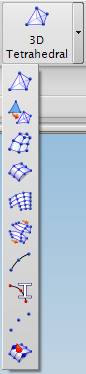
5. Prepare the Finite Element mesh. Select the type of mesh to be created from the meshing drop-down buttons (see Figure 1). In the Mesh dialog box, input the size or number of elements and select the objects to be meshed. To get an idea of how big the elements will be, press the Boundary Nodes button in the Preview panel at the bottom of the meshing dialog box. If the element size is satisfactory, press “OK” to accept the mesh choices.

When meshing, choose the simplest type of element you can use to get the answers you need. Beams should generally be modeled using beam elements, not solid elements. Similarly, sheet or plate-like structures should be modeled using shell elements, not solid elements. In general, use the following types of elements.

· For long and slender structures of constant cross-section, use 1-D beam elements ().

· For thin wall structures of constant thickness (plates and shells), use 2-D shell elements ().

· For complex, thick structures that are not uniform in any direction, use 3-D solid elements ( or ).

Figure 1. Meshing Drop-down Buttons.	Figure 2. Constraint Type Drop-down Buttons.	Figure 3. Load Type Drop-down Buttons.

As well, choose the simplest kind of space to model the situation.

· If the part is flat (like a plate) with constant thickness and all the loads are in the plane of the part, then use 2-D plane stress elements (the out-of-plane stress is zero).

· If the part is prismatic and very long with constant cross-section (like a dam) and all the loads are in the plane of the cross-section and constant along the length, then use 2-D plane strain elements (the out-of-plane strain is zero).

· If the part is axisymetric and all the loads are axisymetric and distributed completely around the circumference (ring loads or pressure loads), then use 2-D axisymetric elements.

6. Create a new simulation.

a) Right-click on the finite element model (“fem1.fem”) in the Simulation Navigator and select “New Simulation…” in the drop-down menu.

b) In the “New Part File” dialog, select the first row (“NX Nastran Sim”). If desired, type in a different file name and select a different directory. Press “OK.”

c) In the “New Simulation” dialog, make sure that the finite element model to which the simulation will apply is correct (Associated FEM) and press “OK.”

d) In the “Solution” dialog, verify that the “NX Nastran” is the Solver, “Structural” is the Analysis Type, and “SESTATIC 101 – Single Constraint” is the Solution Type. Also, make sure Element Iterative Solver is checked if solid elements were used. Press “OK.”

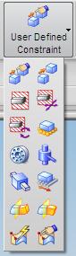
7. Prescribe supports on the structure.

a) Click on the “Constraint Type” button on the toolbar (see Figure 2) and select the type of constraint to be applied (e.g., “Fixed Constraint”). Select the geometry to be restrained and press “OK” in the Constraint dialog when done. After pressing “OK”, small dark blue Xs will appear on the model to show where the constraints have been applied.

Add constraints that are as realistic as possible. E.g., if the A-shaped part in Figure 4 sits freely on the ground with negligible friction and a downward vertical force applied to the top, then it should only be constrained in the Y direction at the two points shown. This is because, as the bottom spreads, only the two inside corners will remain in contact with the ground and the other points will lift a small amount.

(a) (b)

Figure 4. B.C. constrains contact points in the Y direction only – Correct behavior

For this problem, do not add boundary constraints that restrict this upward deflection, as shown in Figure 5. This will yield inaccurate results that make the structure seem stiffer than it really is, and stress concentrations will not appear in the correct places. Also, do not add boundary conditions that also restrict movement in the X direction. Then the results will be inaccurate, as shown in Figure 6. Do not add unrealistic rotational constraints, as shown in Figure 7. Figures 5, 6 and 7 each will have less deflection at the top than Figure 4. Be aware of which kind of situation you have.

(a) (b)

Figure 5. B.C. constrains all of bottom in the Y direction – Incorrect behavior

(a) (b)

Figure 6. B.C. constrains in the X and Y direction – Incorrect behavior

(a) (b)

Figure 7. B.C. constrain X, Y translation and rotation – Incorrect behavior

b) Add enough restraints to avoid rigid body motion – there must be sufficient boundary conditions to keep the part from accelerating ad infinitum. Normally you would add a constraint in the X direction in one place as shown in Figure 8(a). If you do not, the body will tend to accelerate as shown in Figure 8(b). This is will happen even if there are no forces in the X direction. This is true numerically, due to modeling, truncation and rounding errors. This is also true in real life, under ideal conditions, since any small force could send the body moving.

Because of this requirement, you will notice that Figure 4 is not quite correct, since it DOES allow rigid body motion.

(a) (b)

Figure 8. Add sufficient constraints to avoid rigid body motion – (a) is correct (b) is accelerating ad infinitum

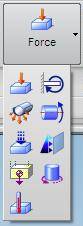
8. Prescribe loads.

a) Click on the “Load Type” button on the toolbar (see Figure 3) and select the type of load to apply. Loads can be forces acting on a point, pressure forces acting on a surface, or body forces such as gravity acting over the entire volume. Other loads such as moments and bearing loads can also be applied. Choose the type of load that is the most representative of your situation.

b) Select the location to receive the load. Type in the magnitude and select the direction of the load (if applicable). Press “OK” for the dialog when done.

9. Solve the Finite Element problem.

a) In the Simulation Navigator right-click on “Solution 1” and select “Model Setup Check” in the drop-down menu. A text window will open up indicating whether there are any errors in the setup of the problem. If there are errors or warnings, go back to previous steps to resolve the error. Otherwise just close the window.

b) In the Simulation Navigator right-click on “Solution 1” and select “Solve…” in the drop-down menu.

c) In the “Solve” dialog click the “OK” button.

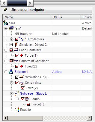
d) Wait for the solution to be calculated. After it is finished, the Results item should appear in the bottom of the Solution Navigator as shown in Figure 9. All of the windows that popped up can then be closed.

Figure 9. Solution Navigator with Results Computed.	Figure 10. Post-Processing Navigator.

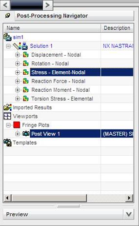
10. View the results.

a) In the Simulation Navigator double-click on Results to bring up the “Post-Processing Navigator” shown in Figure 10.

b) Check the correctness of the displacements.

a. Expand “Solution 1” and double-click on “Displacement – Nodal”. Areas in red have high displacements while the areas shown blue have small or no displacements.

b. To show the undeformed shape at the same time as the deformed results, double-click on “Post View 1” in the “Post-Processing Navigator.” In the “Post View” dialog, check “Show undeformed model” as shown in Figure 11 and press “OK.”

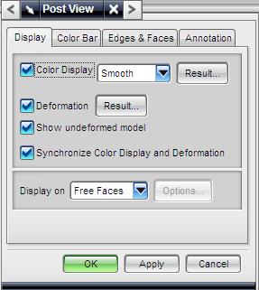
Figure 11. Post View Dialog

c. Look at the restraint locations to verify that there are no incorrect deflections of the structure at the restraints. If necessary, correct or re-input the restraint condition.

c) Check the correctness of the stresses.

a. In the “Post-Processing Navigator” expand “Stress – Element-Nodal” and double-click on a stress of interest for which you know approximately what the value should be (e.g., “XX” for s_x, “YY” for s_y, or “XY” for t_xy).

b. Look at places where pressure loads have been applied normal to a surface. At these points, the stress in the part, in the direction normal to the surface, should closely match the applied pressure. To observe stresses at specific node locations turn on the “Post-Processing” tool bar and press the “Identify” button. Moving the mouse over a node will show the stress at that node for the given element. Clicking on a node will send the information to the “Identify” dialog box.

c. Compare the FEA results with your hand calculations (or experimental results) to verify that there are no major errors in entering data. The numerical results and the hand calculations should be in the same ball park (same order of magnitude). If they are not, some data may have been entered incorrectly or the hand calculations are incorrect. Either problem needs to be resolved.

d) Observe the quantity of interest, corresponding to the failure mode of interest.

Display the correct type of result for the failure mode you are studying. If you are concerned about:

· brittle fracture à show max principle stresses;

· ductile fracture à show von Mises stresses;

· too much deflection à show displacements; etc.

11. Refine the mesh until the results converge.

a) Return to the FEM file (use the Window menu).

b) In the “Simulation Navigator” expand the collectors for the mesh, and double click on the mesh. In the meshing dialog, reduce the size of the elements from Step 5 and save the FEM file.

c) Return to the SIM file (using the Window menu).

d) Repeat Steps 9 and 10.

e) Observe the change in verifiable quantities (e.g., s_x at point from hand calculation) and quantities of interest (e.g., maximum stress, deflection at point of interest).

f) Repeat Steps (a) to (e) until the change in the quantity is less than the error you are willing to accept.

Beware of sources of infinite stress, as shown in Figure 12(a). Mathematically, these points must converge to infinity. Therefore the results will not be realistic in that region. (They should be realistic away from that region.) If you want to avoid infinite stresses, distribute point loads as pressures, round sharp corners, etc., as shown in Figure 12(b).

(a) (b)

Figure 12. Places with stress concentrations will converge to infinite stress as the mesh becomes finer.

12. Make some conclusions from the results. Will the part fail under the given conditions? Is the highest stress less than the yield stress? What is the factor of safety?